What Postgres knows about your tables

When a query is slow, the instinct is to run EXPLAIN against it. The planner answers the question that matters: will it use an index or read the whole table, how many rows does it expect, which join order does it pick. That output is the most useful single artifact in query tuning.

But EXPLAIN needs something you do not always have — a live connection to the database, with the right schema and production-like statistics. In an observability setting that is often exactly what you lack. You are looking at a query that ran twenty minutes ago, on a database you watch but do not operate. There is no open session to run anything against, and even if there were, running planner experiments against a production primary during an incident is not a casual thing to do.

So the question is whether you can reproduce the useful part of EXPLAIN — the structural decisions — offline, from data collected ahead of time, with the database out of the loop. The answer is mostly yes, and the reason it works is that the planner is not magic. It is a function. Its inputs are the query and a specific, enumerable set of statistics about your tables. Both are things you can capture in advance. Our platform shows a query's likely plan this way, without ever opening a connection back to the database at the moment you ask. This post is about the inputs that make that possible, because they are worth knowing whether or not you ever build the prediction step yourself.

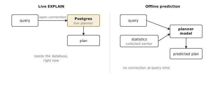
The same plan, reached two ways. The live planner reads statistics from inside the running server; an offline model reads the same statistics from a copy collected earlier. Only the cost model and the live system state differ between them — a difference the closing section returns to.

The first input: the query, parsed by Postgres's own parser

You cannot reason about a SQL statement by matching patterns against the text. WHERE clauses, subqueries, joins, aliases, casts, function calls — SQL has enough surface area that regex-based parsing breaks the moment a query gets interesting. You need a real parse tree.

The parser does not have to come from a running server. pganalyze maintains libpg_query, which vendors the actual parser source from the PostgreSQL server and compiles it to run standalone, with bindings for several languages. It is the same grammar the server uses — the same keywords, the same precedence, the same node types — running outside a database process. sqlc, DuckDB, and GitLab lean on it for the same reason: to understand Postgres SQL, use Postgres's parser.

Feed it a statement and you get a structured tree: a SELECT with its from-clause, where-clause, sort-clause, target list, and so on, down to the leaves. From that tree you can extract, reliably, which tables the query reads and how aliases map back to real names; the columns in the WHERE clause and — this is the part that matters most — how each one appears; the join conditions; the order-by columns; and whether there is a LIMIT or an aggregate.

The shape of a predicate decides everything downstream. created_at > $1 can use an index on created_at. date(created_at) = $1 cannot, because the index stores created_at, not date(created_at). The two differ by one function call, and the parse tree is what lets you tell them apart exactly instead of guessing. That is one input. The other is the statistics, which is the part most engineers have never looked at directly.

The second input: what Postgres records about your data

Whenever ANALYZE runs — automatically through autoanalyze once a table has changed enough, or by hand after a bulk load — Postgres samples a bounded number of rows from each table, governed by default_statistics_target, and writes down a compact statistical summary. At planning time the planner reads only this summary, never your actual rows. Collect the same summary and you are holding the same inputs the planner holds. It lives in a few catalogs, all queryable as ordinary SQL.

Table size comes from pg_class:

SELECT relname, reltuples, relpages
FROM pg_class c JOIN pg_namespace n ON n.oid = c.relnamespace
WHERE c.relkind = 'r' AND n.nspname = 'public';

reltuples is the estimated live row count; a value of -1 means the table has never been analyzed, so treat it as unknown. relpages is the size in blocks — 8 KB each on a default build. Row count is the multiplier behind every estimate — everything downstream is some fraction of reltuples.

Two notes before the rest. relkind = 'r' selects ordinary tables only. A declaratively partitioned table's parent has relkind = 'p' and stores no data pages of its own: relpages is always 0, and reltuples stays at -1 unless you run ANALYZE on the parent by hand, since autoanalyze skips partitioned parents. And the public-schema filter here, repeated in the two queries below, is only for brevity; on a real database drop it or use NOT IN ('pg_catalog', 'information_schema') to cover every application schema.

Index definitions come from pg_indexes, where indexdef is the full reconstructed CREATE INDEX statement:

SELECT indexname, tablename, indexdef
FROM pg_indexes WHERE schemaname = 'public';

From that one string you can read the access method (btree, gin, gist, brin, hash), the column list and its order, whether the index is unique, and any partial-index predicate. Column order is not a detail: an index on (user_id, created_at) is a different tool from one on (created_at, user_id).

Column types and nullability come from information_schema.columns. And the heart of it is pg_stats, a readable view over the table where ANALYZE stores its per-column summary:

SELECT tablename, attname, null_frac, avg_width, n_distinct,
       correlation, most_common_vals, most_common_freqs, histogram_bounds
FROM pg_stats WHERE schemaname = 'public';

Each field earns its place:

• null_frac — fraction of the column that is NULL. The planner uses it to discount estimates and to drive IS NULL and join selectivity.
• avg_width — average value width in bytes, which feeds row width and from there memory and I/O cost.
• n_distinct — the distinct-value count. A positive number is a literal count; a negative number is a ratio of the row count, so -1 means every value is unique. It sets equality selectivity for values that are not among the common ones.
• most_common_vals — the most frequent values, used for exact equality selectivity on common values.
• most_common_freqs — the frequency of each common value, aligned with the list above; these are the selectivity numbers themselves.
• histogram_bounds — boundaries dividing the remaining values into equal-frequency ranges, used for range and inequality selectivity.
• correlation — how closely physical row order matches sorted column order, from -1 to +1. It drives index-scan cost: ordered data reads cheaply, scattered data does not.

The detail worth pausing on is the negative n_distinct, because it trips people up and because understanding it is the difference between treating the statistics as a snapshot and treating them as a description. A positive number is a literal distinct count. A negative number is a fraction of the row count, chosen so the value stays correct as the table grows: -1 on a primary key means "always unique," -0.5 means "distinct count is half the rows." That sign convention is exactly why the statistics are portable — they describe the column's shape, not a frozen count of today's rows. How many common values and histogram buckets you get is governed by default_statistics_target, 100 by default; raise it for finer-grained estimates at the cost of a slower ANALYZE.

Putting them together: the arithmetic the planner runs

With a parsed query and the same statistics the planner reads, the estimates follow from one principle:

estimated_rows = reltuples × selectivity

where selectivity is the fraction of rows a condition keeps. PostgreSQL's documentation works these examples, and they are worth reproducing because they are the actual arithmetic rather than a summary of it (Row Estimation Examples).

For equality where the value is one of the common values, read its frequency straight off the list:

WHERE stringu1 = 'CRAAAA'
most_common_vals  = {EJAAAA, BBAAAA, CRAAAA, ...}
most_common_freqs = {0.00333, 0.003,  0.003,  ...}

selectivity = 0.003
rows = 10000 × 0.003 = 30

For equality where the value is not in that list, assume it is one of the leftover distinct values, spread evenly:

selectivity = (1 − sum(common_freqs)) / (n_distinct − num_common)

with sum(common_freqs) = 0.0303, n_distinct = 676, num_common = 10:
selectivity = (1 − 0.0303) / (676 − 10) ≈ 0.00146
rows = 10000 × 0.00146 ≈ 15

For a range or inequality, find which histogram bucket the value lands in, then count the whole buckets below it plus the fractional position inside its own bucket:

WHERE unique1 < 1000
histogram_bounds = {0, 993, 1997, 3050, ... , 9995}   (10 buckets)
1000 falls in the second bucket (993–1997)

selectivity = (1 + (1000 − 993)/(1997 − 993)) / 10 = 0.1007
rows = 10000 × 0.1007 ≈ 1007

(These figures are the PostgreSQL docs' own example, sampled at a lower statistics target, so the histogram shows ten buckets rather than the default hundred; the bucket-counting works the same at any target.)

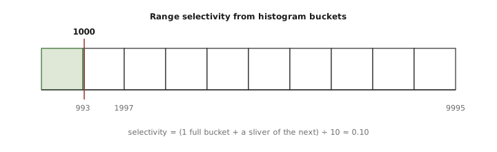
Each bucket holds the same fraction of the rows. The bound at 1000 clears the first of the ten buckets and reaches under one percent into the second — drawn a little wider than scale here so it stays visible — so the selectivity is just over one bucket in ten. (When the data is skewed rather than uniform, the value gaps between boundaries vary, but the bucket-counting stays the same.)

Conditions joined by AND are assumed independent and multiplied together, which is also where the estimate goes wrong on columns that are in fact correlated:

WHERE unique1 < 1000 AND stringu1 = 'xxx'
selectivity = 0.1007 × 0.00146 ≈ 0.000147
rows = 10000 × 0.000147 ≈ 1

And a join on equality is driven by the distinctness of the larger side: selectivity = (1 − null_frac₁)(1 − null_frac₂) / max(n_distinct₁, n_distinct₂), where each n_distinct is the resolved absolute count — abs(n_distinct) × reltuples wherever it is stored as a negative ratio — applied to the product of the two row counts. With a row estimate in hand, the scan decision follows the planner's logic qualitatively. No usable predicate means a sequential scan over the whole table. A predicate whose columns match the leading edge of a btree index means an index scan — leading edge being the operative phrase, since an index on (user_id, created_at) serves a filter on user_id, or on both, but not on created_at alone. A predicate that matches a tiny fraction of a large table makes the index scan overwhelmingly likely; a predicate that matches most of the table often pushes the planner back to a sequential scan, because scattered index reads across most of the pages cost more than reading them in order. That last decision is where correlation earns its keep.

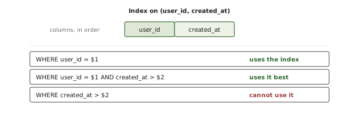
A composite btree is sorted by its first column, then the second within each first. A filter that names the leading column can seek into it; a filter that names only a later column has no starting point and falls back to a sequential scan.

The same statistics, turned into warnings

The row estimates are useful, but the data is arguably more valuable for catching structural mistakes — the cases where a query cannot use an index it looks like it should, which is most of what a "why is this slow" investigation is actually chasing. Flagging these needs the parse tree and the index list, not a precise cost model:

• A function wrapping an indexed column. WHERE date(created_at) = $1 quietly disables the created_at index. The parse tree shows the function; the index list shows the bare-column index that will go unused. The fix is a matching expression index or a rewrite that leaves the column bare.
• A predicate on a column with no index at all, on a table large enough for it to matter. That is a missing index, stated plainly.
• A predicate that does not imply a partial index's condition. A partial index defined … WHERE deleted_at IS NULL is invisible to a query whose own WHERE never mentions deleted_at. The parse tree carries the query's predicates and the index list carries the partial condition, so the mismatch is mechanical to spot.
• A sequential scan on a large table, caught by crossing reltuples against the predicted scan type.
• An OR across columns where only one side is indexed, forcing a scan the indexed side could have avoided.
• A leading-wildcard LIKE '%foo', which a btree index cannot serve — the fix is a trigram index (pg_trgm, GIN or GiST) on the column.

The collected schema outlives any single query, too. The same data supports index recommendations, detects schema drift over time, and surfaces tables whose statistics have gone stale — a reltuples of -1, or a last-analyze timestamp far enough in the past that the estimates above are running on numbers nobody should trust.

Where the honesty goes

An offline prediction is not the same as running EXPLAIN, and the difference is worth stating precisely rather than waving at. Several things the real planner has are not in the statistics at all.

The cost model is the first. Postgres weighs estimated rows against a set of cost constants — sequential and random page-read costs, the per-tuple and per-operator CPU costs, the parallel-worker costs — together with planner parameters like effective_cache_size, which estimates how much memory is available for caching and adjusts the cost of repeated index reads rather than acting as a cost unit itself. The combination is what turns a row estimate into a number it can compare across plans. Live cache state is the second: whether the pages a scan needs are already in shared buffers or the operating system cache changes the real cost from one minute to the next, and no static summary captures that. Cross-column correlation is the third — plain pg_stats is per-column, so the independence assumption behind multiplying selectivities can be badly wrong on columns that move together, which is the same blind spot the real planner has until you create extended statistics to cover it. And the runtime context is the fourth: the actual bound parameter values, generic versus custom plans for prepared statements, and session settings all steer the live planner in ways a static analysis does not see.

So the honest claim is a narrow one. An offline analyzer gets the structural answer right — which columns are involved, which indexes exist on them, whether the query is shaped so Postgres can use them, and a row estimate in the right order of magnitude. That is the part of the plan most investigations are trying to recover, and it is recoverable without a connection. The exact cost, the join order chosen under contention, the effect of a cold cache: those need the running system.

That boundary is the real subject here. The planner's decisions are a function of statistics you can collect and carry around; the planner's costs are a function of a live system you cannot fully reproduce from a summary. Knowing which of your questions falls on which side of that line is most of the skill — and for the common question, the one that starts with a slow query and ends with "could this have used an index," the line falls on the side you can answer with data you already have.

What it buys you

Set against those limits is what the approach gives you for free. It needs no connection, so it runs on the query that already executed, against a database you only monitor — nothing to open, no load placed on a production primary, no chance of aiming a heavy EXPLAIN at the wrong statement in the middle of an incident. It runs after the fact, on the slow query from twenty minutes ago, which is both when you most want an answer and when a live EXPLAIN is hardest to come by. And because it is only a parse tree weighed against a stored summary, it is cheap enough to run across every slow query you have captured instead of the one you happened to check — the focused minute a person spends reading a plan becomes something you can apply in bulk and leave running.

The answers it returns are the ones that close most investigations: which tables are read, whether an index is taken or skipped, why a query that looks indexed is not, and a row count in the right order of magnitude. That is the substance behind most "why is this slow" questions, recovered from statistics you already hold, without waiting for the database to be in the right state to ask. The exact cost stays the planner's to keep. The decision it would reach does not — and the decision is usually what sent you looking.